Dynamic Programming 2 (Shortest Path, DAG)

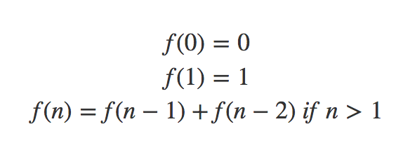
In the first part, we learned about the Fibonacci Number. In this article, we will talk about the shortest path problem and will learn some properties of Dynamic Programming along the way. The shortest path is a graph problem but you don’t really need to know about graph algorithms for this article.

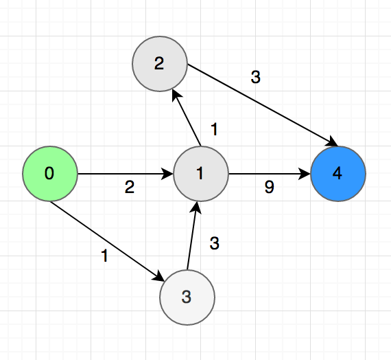
Let’s say we need to find the shortest between one city to another. There are $n$ cities in total, $0$ is the first city and $n-1$ is the last. The path and distance between pairs of cities are marked with arrows like the picture below:

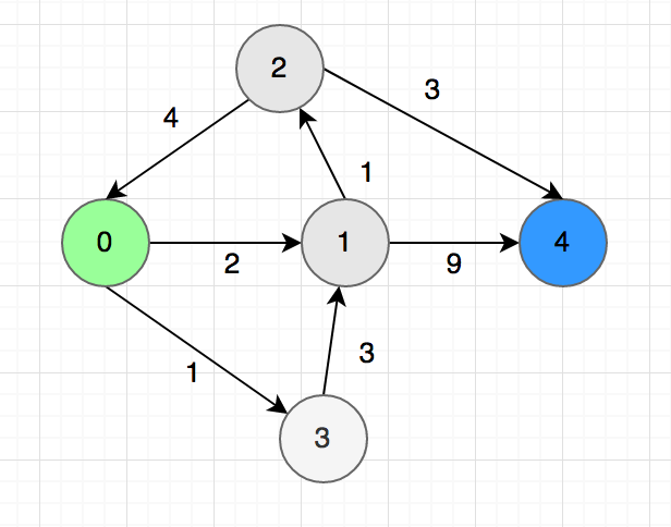
Now we need to find the length of the shortest path between $0$ to $n-1$.

Finding Subproblems/States:

First, we need to find that are the parameters or states can define the problem. Remember the word ‘state’, we will be using it a lot. For this problem, the state is defined by the city you are currently in. Let’s say you are in city $u$, we will express our problem as a function $F(u)$. Just like Fibonacci, we will now try to find a recursive solution.

State Transition and Recursion

We don’t know which is next city to from $u$ to reach the destination in the shortest path. In this step, we will guess the next city and every guess will be a new subproblem. In the graph, we can go to the city $1$ and $3$ from $0$. So we will get the shortest path from $f(0)$ using this formula:

$f(0) = min(f(1) + 2, f(3) + 1)$

The idea is to go to each adjacent city and find the shortest path from there. The answer will bee the minimum of all the guesses. In general:

$f(n – 1) = 0 \\f(u) = min(f(u, v) + w(u, v)) \ where \ (u,v) \in E \ for\ u \ne n – 1$

Here $w(u, v)$ is the distance between $u$ and $v$.

Sub-problem Ordering

Now let’s think about the ordering of the function calls after we run the recursion.

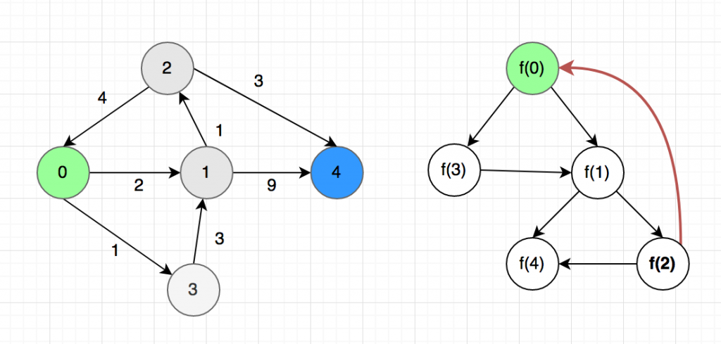
Now we are in big trouble, the subproblems created a cycle. For example, to find the value of $f(0), we need to. know the value of $f(0)$ but $f(2) again depends of $f(0)$. If we try to run this as a code, it will stick in an infinite loop. This brings us to the concept of DAG.

Directed Acyclic Graph (DAG)

A DAG or directed acyclic graph is a directed graph with no cycles. A dynamic programming solution will work only if the subproblems create a DAG.

Even though we can’t solve the shortest path problem in a general graph using the formula above, we still can solve it for a DAG. In the graph above, we can remove the $2->0$ arrow and it will become DAG.

The C++ Code

Now we can solve it using DP. The C++ code will be like this:

One interesting fact is, we can still find the shortest path a general graph using DP but we need to add an extra parameter $k$ which indicates the maximum number of edges we are allowed to use. Rings a bell? Yes, that is very similar to the bellman ford algorithm.

Complexity

We have $n$ subproblems in this problem $f(0), f(1)…f(n-1)$. Moreover, for every city $u$, we are going to a maximum of $n$ adjacent cities. Total complexity will be the multiplication of the number of subproblems and the complexity of internal operations which is $O(n^2)$.

Iterative Version

For this problem, writing the iterative version is a bit difficult but possible. For the iterative version, we need to arrange the subproblems in topological order because, in each subproblem, you must make sure you solved the dependant subproblems. For Fibonacci, it was very easy but for this graph, it’s a bit tricky. You can google about topological sorting in a graph, I also discussed in brief here.

For the example above, we will get ${0, 3, 1, 2, 4}$ after sorting. Now you can loop this array in reversed order for building the table. It’s ok if you can’t implement that for this problem, it’s quite complicated and won’t give any advantage. We will learn more about the Iterative version when we learn LIS and knapsack.

Conclusion

So far you have learned:

  • How to define the subproblems
  • How to transit from one subproblem to another to find the optimal solution
  • What is DAG, why DP can’t work if there is a cyclic dependency?

Still not getting confidence? No problem, this just the start, you will be able to solve some problems after you read the next part.

Happy Coding

Dynamic Programming 1 (Fibonacci)

Dynamic Programming may sound intimidating but the concept is quite easy. In dynamic programming, we divide a problem into multiple subproblems and build-up the solutions from that, but we must be careful not to solve one sub-problem more than once. That is dynamic programming in a nutshell. But to understand if a problem can be solved by dynamic programming or not, you need some experience. In this series, we will know what is Dynamic programming and solve some classic dynamic programming problems. I originally wrote the series in Bengali, this is the translated version.

Dynamic programming is a confusing term, especially the ‘dynamic’ part because it’s not really co-relate to how dynamic programming works. Dr. Richard Bellman used this term to save his research grant, strange but true! So don’t waste time trying to find the meaning behind the naming.

One of the pre-requisite to learn dynamic programming is understanding recursion. Also, I hope you know the basics of time and space complexity (Big O notation).

I am using the lecture series of MIT by Dr. Eric Demaine as the reference for this series. You can watch it here.

Dynamic Programming

Dynamic programming is not an algorithm to solve a particular problem. Rather, it’s a problem-solving technique which can be used to solve many kinds of optimization or counting problem. For example Fibonacci, Coin Change, Matrix Chain Multiplication. Dynamic programming is a kind of brute force but it’s a clever brute force. There are many kinds of problems for which dynamic programming is the only known polynomial solution.

Fibonacci Sequence

Fibonacci is not the best example of dynamic programming but it’s the easiest to start with. An Italian Mathmetician created this sequence while observing the production rate of rabbits. The sequence is like this::

0, 1, 1, 2, 3, 5, 8, 13, 21, 34 ….

Except for the first two numbers, every number is the summation of the previous two numbers. Let’s imagine a function $F(n)$ which returns the $n^{th}$ Fibonacci number. If we define it recursively, it will look like this:

The C++ code for this looks like this:

Now we divided $f(n)$ into two smaller subproblems. Do you know the time complexity for this code? If we call $F(5)$ and represent the function calls as a tree, it will look like this:

Except for the base case, every function is calling two other functions. The time complexity is $O(n^2)$ which is not really great, it’s exponential.

You might have noticed that I highlighted $f(3)$ in two places.  This is to show that for calculating $f(5)$ we are calculating $f(3)$ twice which is clearly a waste!

One of the principles of dynamic programming is we won’t solve one subproblem more than once. So what can we do? The answer is caching the results in a table. If we see that we already have the results for a subproblem in the table, we don’t need to call the function again.

The C++ Code

We used an array called $memo$ to save the results. We initialized it with $-1$ to indicate that the table is empty. You need to choose a value that can’t be part of the answer. During every function call, we are first checking if the result exists in the array.

Complexity

Now the complexity of the code becomes $O(n)$ as we have $n$ subproblems and we are solving every subproblem once. Inside the function, all the operations have constant time complexity.

Memoization

The process of saving the result for later use is called ‘Memoization’, another weird terminology. Memoization Came from the Latin word memorandum, there is actually not much difference with memorization. The term was coined by researcher Donald Mitchie.

Iterative Version

The implementation can be iteratively as well. All we need to do is arranging the sub-problems in topological order. That means we need to solve the subproblems which don’t depend on any other subproblems first (base case) and gradually build the results from smaller subproblems.

For Fibonacci, we already know the results of $f(0)$ and $f(1)$. We can save these values in the table first and gradually solve $f(2), f(3) …. f(n)$ in this order.

For solving the Dynamic Programming problem, it’s easier to find recursive formula at first. After that, we can write the code either recursively or iteratively. In fact, it’s easier to write the recursive code, it works almost like magic. The iterative version can be slightly difficult if there is more than one parameter.

But it’s important to understand the iterative version as well because often it provides some chance to save space.  For example, in the code above, you only need the value of the last two entries of the table, so you don’t really need to maintain the whole table.

There are some standard ways to attack dynamic programming problems. Next, we will see some optimization problem which will give us a better idea of the pattern.

(Next Part)