Dynamic Programming may sound intimidating but the concept is quite easy. In dynamic programming, we divide a problem into multiple subproblems and build-up the solutions from that, but we must be careful not to solve one sub-problem more than once. That is dynamic programming in a nutshell. But to understand if a problem can be solved by dynamic programming or not, you need some experience. In this series, we will know what is Dynamic programming and solve some classic dynamic programming problems. I originally wrote the series in Bengali, this is the translated version.
Dynamic programming is a confusing term, especially the ‘dynamic’ part because it’s not really co-relate to how dynamic programming works. Dr. Richard Bellman used this term to save his research grant, strange but true! So don’t waste time trying to find the meaning behind the naming.
One of the pre-requisite to learn dynamic programming is understanding recursion. Also, I hope you know the basics of time and space complexity (Big O notation).
I am using the lecture series of MIT by Dr. Eric Demaine as the reference for this series. You can watch it here.
Dynamic Programming
Dynamic programming is not an algorithm to solve a particular problem. Rather, it’s a problem-solving technique which can be used to solve many kinds of optimization or counting problem. For example Fibonacci, Coin Change, Matrix Chain Multiplication. Dynamic programming is a kind of brute force but it’s a clever brute force. There are many kinds of problems for which dynamic programming is the only known polynomial solution.
Fibonacci Sequence
Fibonacci is not the best example of dynamic programming but it’s the easiest to start with. An Italian Mathmetician created this sequence while observing the production rate of rabbits. The sequence is like this::
0, 1, 1, 2, 3, 5, 8, 13, 21, 34 ….
Except for the first two numbers, every number is the summation of the previous two numbers. Let’s imagine a function $F(n)$ which returns the $n^{th}$ Fibonacci number. If we define it recursively, it will look like this:
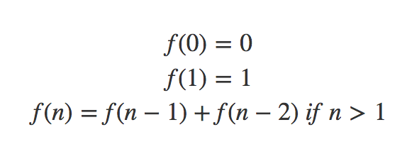 The C++ code for this looks like this:
|
1 2 3 4 5 6 |
int f(int n) { if (n == 0) return 0; if (n == 1) return 1; return f(n - 1) + f(n - 2); } |
Now we divided $f(n)$ into two smaller subproblems. Do you know the time complexity for this code? If we call $F(5)$ and represent the function calls as a tree, it will look like this:
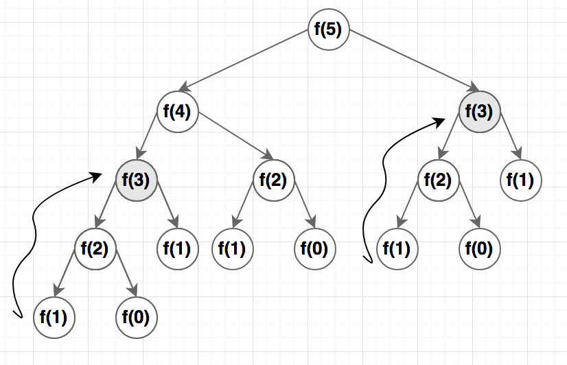
Except for the base case, every function is calling two other functions. The time complexity is $O(n^2)$ which is not really great, it’s exponential.
You might have noticed that I highlighted $f(3)$ in two places. This is to show that for calculating $f(5)$ we are calculating $f(3)$ twice which is clearly a waste!
One of the principles of dynamic programming is we won’t solve one subproblem more than once. So what can we do? The answer is caching the results in a table. If we see that we already have the results for a subproblem in the table, we don’t need to call the function again.
The C++ Code
|
1 2 3 4 5 6 7 8 9 10 11 12 13 14 15 16 17 18 19 20 21 22 |
#define MAX_N 20 #define EMPTY_VALUE -1 int memo[MAX_N]; int f(int n) { if (n == 0) return 0; if (n == 1) return 1; if (memo[n] != -1) { return memo[n]; } memo[n] = f(n - 1) + f(n - 2); return memo[n]; } void init() { for (int i = 0; i< MAX_N; i++) { memo[i] = EMPTY_VALUE; } } |
We used an array called $memo$ to save the results. We initialized it with $-1$ to indicate that the table is empty. You need to choose a value that can’t be part of the answer. During every function call, we are first checking if the result exists in the array.
Complexity
Now the complexity of the code becomes $O(n)$ as we have $n$ subproblems and we are solving every subproblem once. Inside the function, all the operations have constant time complexity.
Memoization
The process of saving the result for later use is called ‘Memoization’, another weird terminology. Memoization Came from the Latin word memorandum, there is actually not much difference with memorization. The term was coined by researcher Donald Mitchie.
Iterative Version
The implementation can be iteratively as well. All we need to do is arranging the sub-problems in topological order. That means we need to solve the subproblems which don’t depend on any other subproblems first (base case) and gradually build the results from smaller subproblems.
For Fibonacci, we already know the results of $f(0)$ and $f(1)$. We can save these values in the table first and gradually solve $f(2), f(3) …. f(n)$ in this order.
|
1 2 3 4 5 6 7 8 9 10 11 12 13 |
#define MAX_N 20 int memo[MAX_N]; int f(int n) { memo[0] = 0; memo[1] = 1; for(int i = 2;i < n;i++) { memo[n] = memo[i - 1] + memo[i - 2]; } return memo[n]; } |
For solving the Dynamic Programming problem, it’s easier to find recursive formula at first. After that, we can write the code either recursively or iteratively. In fact, it’s easier to write the recursive code, it works almost like magic. The iterative version can be slightly difficult if there is more than one parameter.
But it’s important to understand the iterative version as well because often it provides some chance to save space. For example, in the code above, you only need the value of the last two entries of the table, so you don’t really need to maintain the whole table.
There are some standard ways to attack dynamic programming problems. Next, we will see some optimization problem which will give us a better idea of the pattern.
One Comment